




- 20 Jul, 2026
- Verification & Validation
Most small-aircraft “design” you find online is a spreadsheet of plausible-looking numbers nobody re-derives. FT-1 — the fixed-wing airframe that joins the quadrotor from L2 onward in the Robavionix curriculum — was built under a different rule: every geometric and mass number has to trace to a formula, a cited method, or a real solver run. This post is that trace, including the two places the model itself found a real problem — and, further down, a second and completely independent tool chain built to check the first one’s most important finding.
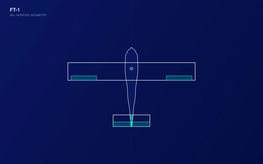
Both drawings are rendered directly from the coordinates in ft1.avl, not sketched — the fuselage outline is the one explicitly-flagged exception, still illustrative pending a finished cross-section.
Sizing from first principles, not a spreadsheet
Wing area comes from a wing-loading target (a conceptual-design sizing choice, not a derived quantity) and is checked against stall speed directly from the lift equation: at 0.45 m², 2.0 kg design mass, and an assumed CL_max of 1.2, V_stall ≈ 7.7 m/s, giving a 1.69× margin over the 13 m/s cruise target. Tail sizing uses the tail-volume-coefficient method standard in aircraft conceptual design texts (Raymer’s Aircraft Design: A Conceptual Approach is the usual reference for the typical coefficient ranges by aircraft class) — a horizontal tail volume of 0.55 and vertical of 0.035, both within the ranges cited for light/general-aviation-class aircraft.
A geometry that actually loads — and the bug that proved the point
Simulink line drawings are cheap to fake. An AVL model either loads or it doesn’t. Running the real geometry file through AVL 3.40 (Drela & Youngren, MIT — originally written by Youngren circa 1988 for MIT’s Athena software collection, extensively developed since) surfaced a real bug on the first attempt: a multi-line source-attribution comment placed before the Clark-Y airfoil coordinates (pulled directly from the UIUC Airfoil Coordinates Database) broke AVL’s line reader, which accepts exactly one title line before numeric data. Four airfoil reads failed silently before the fix.
Once fixed, the same run exposed something more consequential: the design’s nominal 25%-MAC CG target produced a static margin of 24.3% against the neutral point AVL actually computed — nearly double the 10–15% design target. The correction wasn’t cosmetic: solving for the CG that hits the top of the target band moved the reference point 23 mm aft, back into the range the airframe’s battery-bay slide margin was sized to absorb. Static margin after the correction: 14.97%.
Mass and inertia, checked two independent ways
Small-UAV mass properties don’t come from a lookup table the way tail volume does — full-scale statistical weight-fraction methods don’t hold at this scale. The standard approach is component buildup: sum actual or estimated part masses at known positions, approximate each as a simple shape, and apply the parallel axis theorem. FT-1’s six-component breakdown treats the battery position as the one free variable that closes the loop — solving the mass-moment equation for the CG found above places it at 0.2825 m, between the wing and the target CG, which is where a battery tray on this layout would physically sit.
The resulting inertia (Ixx = 0.1507, Iyy = 0.0928, Izz = 0.2392 kg·m²) was computed by hand via parallel-axis summation and independently recomputed by AVL after loading the resulting mass file — the two agree to three or four significant figures. As a sanity check with real physical content: roll inertia is 99.6% wing-contributed, which is exactly what should happen when most of the mass sits within 25 cm of the fuselage centerline and the wing spans ±90 cm either side of it.
The eventual empirical check — measuring the built airframe’s actual inertia — will use a bifilar pendulum, a standard technique for small aircraft with a specific optimized-measurement procedure published in Jardin & Mueller, “Optimized Measurements of Unmanned-Air-Vehicle Mass Moment of Inertia with a Bifilar Pendulum,” Journal of Aircraft, Vol. 46, No. 3 (2009), pp. 763–775.
Running the eigenvalues, and reporting what they actually say
With a trimmed run case (CL = 0.4212 at 13 m/s, elevator deflection just 0.75° — nowhere near saturated), AVL’s MODE command produces the linearized dynamic modes directly, checked against the Level 1 flying-qualities criteria in MIL-F-8785C, Military Specification: Flying Qualities of Piloted Airplanes (1980) — the same reference this curriculum already cites for the fixed-wing verification criteria.
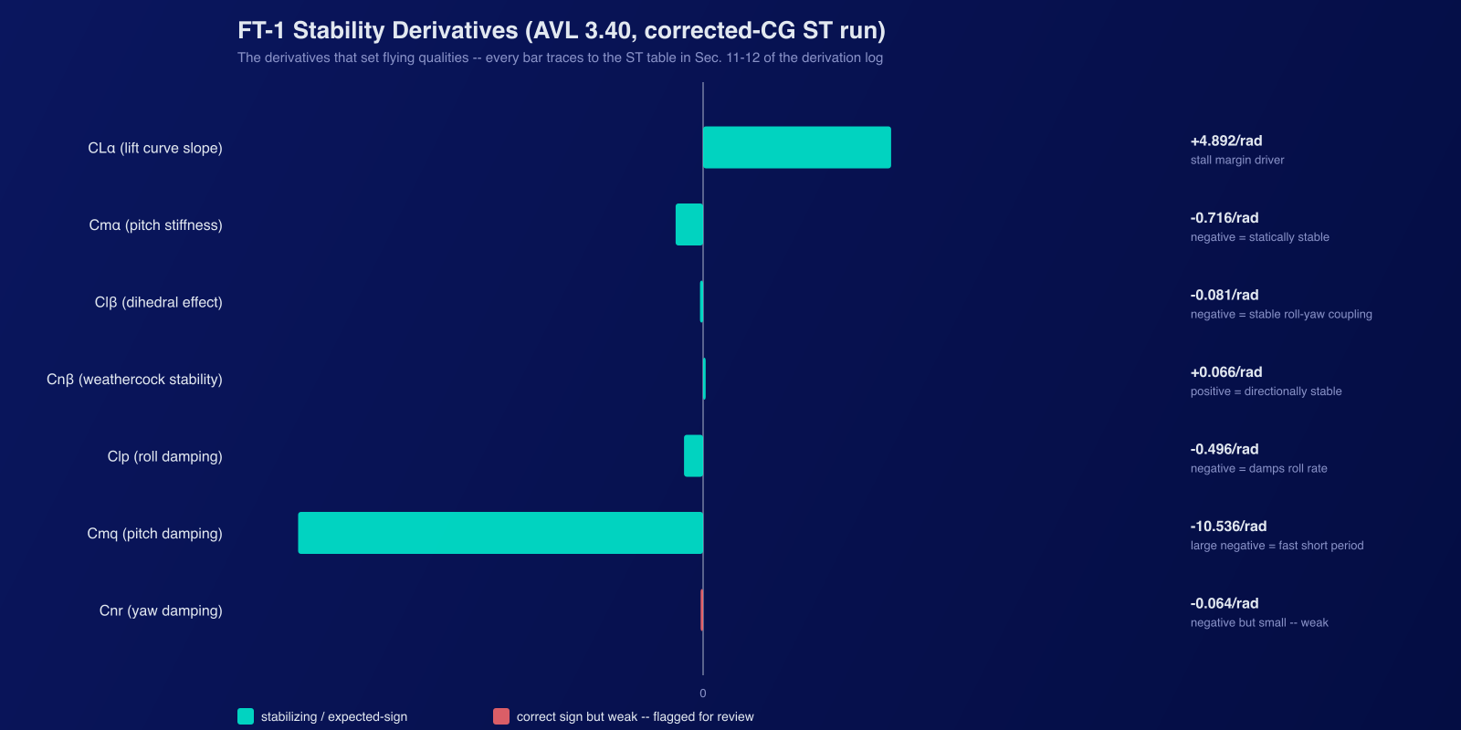
These are the numbers the five dynamic modes below actually come from — not tuned to hit a target, just what AVL’s vortex-lattice solver returns for this geometry and mass distribution. Every one has the sign a stable airframe needs except Cnr, which is correctly signed but weak — flagged here rather than left implicit, and it turns out to matter (see the spiral mode, below).
Three modes came in clean: roll subsidence (0.063 s time constant, well inside the ≤1.0 s ceiling), Dutch roll (ωn = 5.12 rad/s, ζ = 0.181, inside the target band), and short period (ζ = 0.769, close to target). Two did not, and both are reported here rather than edited out:
- Spiral mode is divergent, and faster than intended — a 12.4 s amplitude-doubling time against a >30 s design target and MIL-F-8785C’s own 20 s Category B floor.
- Phugoid damping is an order of magnitude below spec — ζ = 0.0044 against a Level 1 floor of 0.04. The mode is stable but barely damped at all, plausibly because the current model still has zero viscous drag (the XFOIL polar hasn’t been run yet, so CDvis = 0 throughout).
Neither is disqualifying at this stage — both are exactly the kind of finding a verification pass is supposed to produce — but presenting five-for-five when the real number is three-for-five would defeat the entire point of building something checkable in the first place.
Two solvers, one aircraft: cross-validating with Simulink
Everything above comes from one tool chain: AVL. A real result computed once is still a result computed once. So the next step was building a second, structurally different check — trim, linearize, and run a nonlinear open-loop disturbance test in Simulink — and seeing whether it agrees with AVL without being told the answer in advance.
Rather than build that from scratch, it reuses a nonlinear 6DOF Simulink architecture already built and flight-relevant for a different fixed-wing airframe from the author’s own prior research. Inspecting the block diagram (not reading source that doesn’t exist for a compiled .slx, but tracing actual block parameters) showed the whole aerodynamic and mass model is parameter-driven: every derivative, every mass and inertia term, every reference length is read from a named workspace variable, with no aircraft-specific logic baked into the blocks themselves. That means reusing it for FT-1 needed zero block-diagram edits — only a new script defining the same variable names with FT-1’s real numbers.
The one real design decision was a control-surface mismatch: the reused harness has five named actuator slots (flap, flap2, aileron, elevator, elevator2); FT-1 has four real surfaces (aileron, elevator, elevator2, rudder). Aileron, elevator, and elevator2 map straight across by name. The flap slot was repurposed to carry FT-1’s rudder derivatives; the flap2 slot was zeroed out rather than deleted, and both choices are documented directly in the script, not left implicit.
Trimmed in Simulink via findop, FT-1 settles at essentially the same small-angle, near-zero-alpha cruise point AVL finds — a small, explained gap in elevator trim comes from the Simulink model including the thrust line’s pitching-moment offset from the CG, which AVL’s pure-aerodynamics solver doesn’t model at all. That’s a real physical difference between what the two tools compute, not an error, and it’s reported as one.
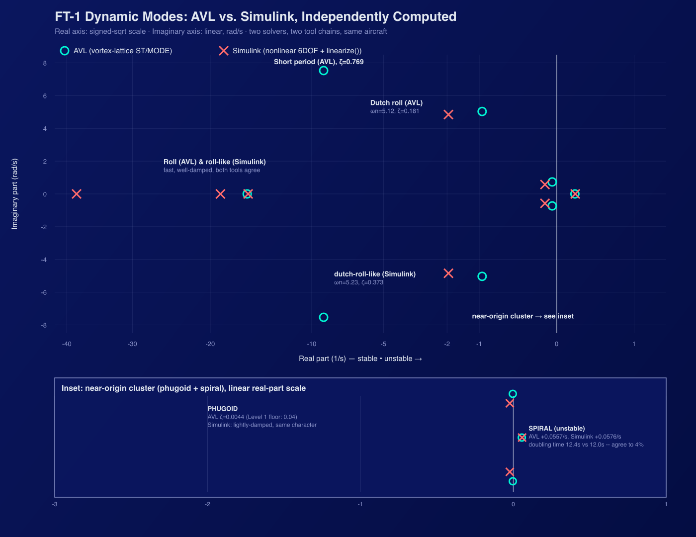
This is the actual point of building a second tool chain: the linearized model’s eigenvalues split cleanly into a longitudinal set, a lateral set, and four exactly-zero modes (position and heading states that don’t feed back into the force/moment equations at this trim point) — and the one number that mattered most from the AVL run shows up again, independently. AVL’s spiral mode has a 12.4 s amplitude-doubling time; Simulink’s linearization, built from a completely different plant model and a different solver, gives 12.0 s — agreement to within 4%, from two tools that share nothing but the same underlying stability derivatives. That is a real cross-check, not the same number computed twice.
The nonlinear time-domain response backs this up directly. Perturbing the trimmed model with a small initial disturbance and integrating the unforced response — no controller, no feedback, actuators held at their trimmed constants — gives a direct test of whether the linearization actually describes the real (nonlinear) aircraft near this operating point:
Both plots use the same disturbance, on the same state, in both models — a linear-vs-nonlinear comparison only means something if the input is actually identical, so getting that matched was a precondition for trusting the rest of the plot, not a detail to gloss over. With that fixed, linear and nonlinear curves sit on top of each other for the full 20-second run, in both the longitudinal case (a small pitch-rate disturbance) and the lateral case (a roll-rate disturbance) — exactly what a correct linearization should produce this close to trim. Roll angle and yaw rate both grow slowly for the full run in both models, the time-domain signature of the same unstable spiral mode the pole map and the original AVL run already found.
The full folder — trim/linearize script, the two linear open-loop harnesses, the nonlinear disturbance test, and every .mat output — lives alongside ft1.avl and ft1.mass, structured to mirror the author’s own prior open-loop verification work rather than invented from scratch for this aircraft.
Why this is the whole point
A teaching platform whose credibility rests on “trust us” doesn’t teach the thing it claims to teach. Every number in this post resolves to a formula you can rerun, a citation you can pull up, an AVL log file that exists on disk, or now a second solver’s independent agreement with the first. The two open problems from the AVL run go into the next design iteration, not into a footnote — and the spiral instability, the more serious of the two, no longer rests on a single tool’s word for it.
References: AVL 3.40, M. Drela & H. Youngren, MIT — User Primer · Clark-Y coordinates, UIUC Airfoil Coordinates Database · MIL-F-8785C, Flying Qualities of Piloted Airplanes (1980) · M. Jardin & T. Mueller, “Optimized Measurements of Unmanned-Air-Vehicle Mass Moment of Inertia with a Bifilar Pendulum,” Journal of Aircraft, 46(3), 2009, pp. 763–775.